Flujo Fraccional de Buckley-Leverett y Método de Welge

Ecuación de avance frontal, saturación de breakthrough y pronóstico de producción

Yacimientos
Producción
Python
R

Implementación completa de la ecuación de flujo fraccional de Buckley-Leverett con el método gráfico de Welge: permeabilidades relativas de Corey, curva de fw, saturación del frente, pronóstico de producción y perfil de saturación.

Author
Published

August 1, 2026

Introducción

En 1942, Buckley y Leverett desarrollaron un modelo para describir el desplazamiento inmiscible de un fluido por otro en un medio poroso — la base teórica de toda inyección de agua. El modelo asume fluidos incompresibles, sistema homogéneo y flujo unidimensional, ignorando los efectos de presión capilar y gravedad.

La solución nos da el perfil de saturación a lo largo del yacimiento y permite calcular cuándo llega el agua al pozo productor (breakthrough), cuánto aceite se recupera, y cómo se comporta la producción después.

¿Por qué es importante?

Es el fundamento de todo diseño de inyección de agua. Sin entender Buckley-Leverett, no puedes evaluar si un waterflood va a funcionar ni cuánto aceite vas a recuperar.

Video

Ecuación de Flujo Fraccional

El flujo fraccional de agua (\(f_w\)) se define como la fracción del flujo total que es agua:

\[f_w = \frac{q_w}{q_o + q_w}\]

Aplicando la ley de Darcy para flujo simultáneo de aceite y agua en un sistema horizontal (sin gravedad ni presión capilar):

\[f_w = \frac{1}{1 + \frac{k_{ro} \cdot \mu_w}{k_{rw} \cdot \mu_o}}\]

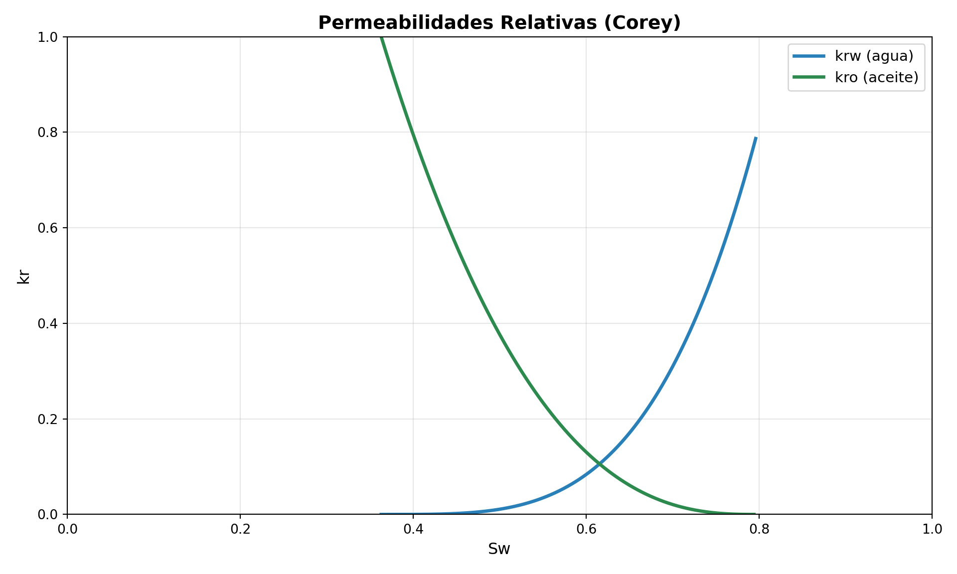
Las permeabilidades relativas se modelan con las ecuaciones de Corey:

\[k_{ro} = k_{ro,max} \cdot (1 - S_{wD})^{n_o}\]

\[k_{rw} = k_{rw,max} \cdot S_{wD}^{n_w}\]

Con la saturación normalizada:

\[S_{wD} = \frac{S_w - S_{wc}}{1 - S_{or} - S_{wc}}\]

Datos del Ejemplo

Datos del ejemplo.
Parámetro Valor Unidades
Área del yacimiento 6,000 ft²
Longitud 1,000 ft
Porosidad 0.15 fracción
Permeabilidad 100 md
Viscosidad del aceite 2 cp
Viscosidad del agua 1 cp
Bo 1.2 RB/STB
Bw 1.0 RB/STB
Sor 0.205 fracción
Swc = Swi 0.363 fracción
kromax 1.0
krwmax 0.78
no (Corey aceite) 2.56
nw (Corey agua) 3.72
Gasto de inyección 338 B/D

Paso 1 — Permeabilidades Relativas

Ver código
import numpy as np
import matplotlib.pyplot as plt

# === DATOS DE ENTRADA ===
L = 1000; Ar = 6000; Poro = 0.15; K = 100
VisO = 2; VisW = 1; Bo = 1.2; Bw = 1
Sor = 0.205; Swc = 0.363; Swi = 0.363
kromax = 1.0; krwmax = 0.78
no = 2.56; nw = 3.72
Winj = 338

# === PERMEABILIDADES RELATIVAS ===
Sw = np.arange(Swc, 1 - Sor + 0.001, 0.001)
SwD = (Sw - Swc) / (1 - Sor - Swc)
krw = krwmax * SwD**nw
kro = kromax * (1 - SwD)**no
<string>:1: RuntimeWarning: invalid value encountered in power
Ver código
fig, ax = plt.subplots(figsize=(10, 6))
ax.plot(Sw, krw, '-', lw=2.5, color='#2980b9', label='krw (agua)')
ax.plot(Sw, kro, '-', lw=2.5, color='#2d8a4e', label='kro (aceite)')
ax.set_xlabel('Sw', fontsize=12)
ax.set_ylabel('kr', fontsize=12)
ax.set_title('Permeabilidades Relativas (Corey)', fontsize=14, fontweight='bold')
ax.legend(fontsize=11); ax.grid(True, alpha=0.3)
ax.set_xlim(0, 1); ax.set_ylim(0, 1)
(0.0, 1.0)
(0.0, 1.0)
Ver código
plt.tight_layout(); plt.show()
Figure 1: Curvas de permeabilidad relativa de Corey para el sistema agua-aceite.
Ver código
library(ggplot2)

L=1000; Ar=6000; Poro=0.15; K=100
VisO=2; VisW=1; Bo=1.2; Bw=1
Sor=0.205; Swc=0.363; Swi=0.363
kromax=1; krwmax=0.78; no=2.56; nw=3.72
Winj=338

Sw <- seq(Swc, (1-Sor), 0.001)
SwD <- (Sw - Swc) / (1 - Sor - Swc)
krw <- krwmax * SwD^nw
kro <- kromax * (1 - SwD)^no

ggplot() +
  geom_line(aes(x=Sw, y=krw, color="krw (agua)"), linewidth=1.2) +
  geom_line(aes(x=Sw, y=kro, color="kro (aceite)"), linewidth=1.2) +
  scale_color_manual(values=c("krw (agua)"="#2980b9", "kro (aceite)"="#2d8a4e")) +
  labs(x="Sw", y="kr", title="Permeabilidades Relativas (Corey)", color="") +
  xlim(0, 1) + ylim(0, 1) + theme_minimal() +
  theme(plot.title=element_text(face="bold", size=14))
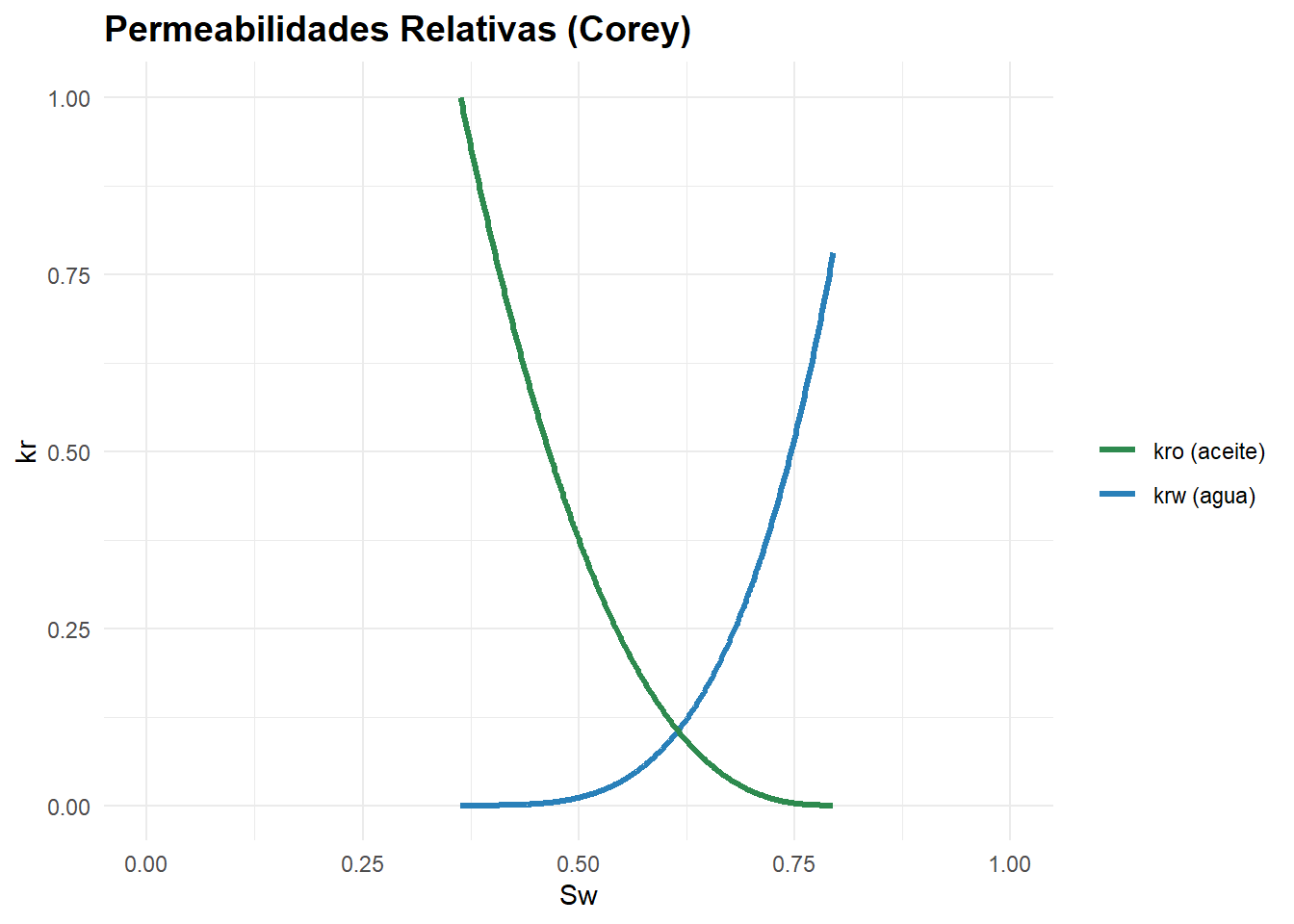
Figure 2: Curvas de permeabilidad relativa de Corey.

Paso 2 — Curva de Flujo Fraccional y Tangente de Welge

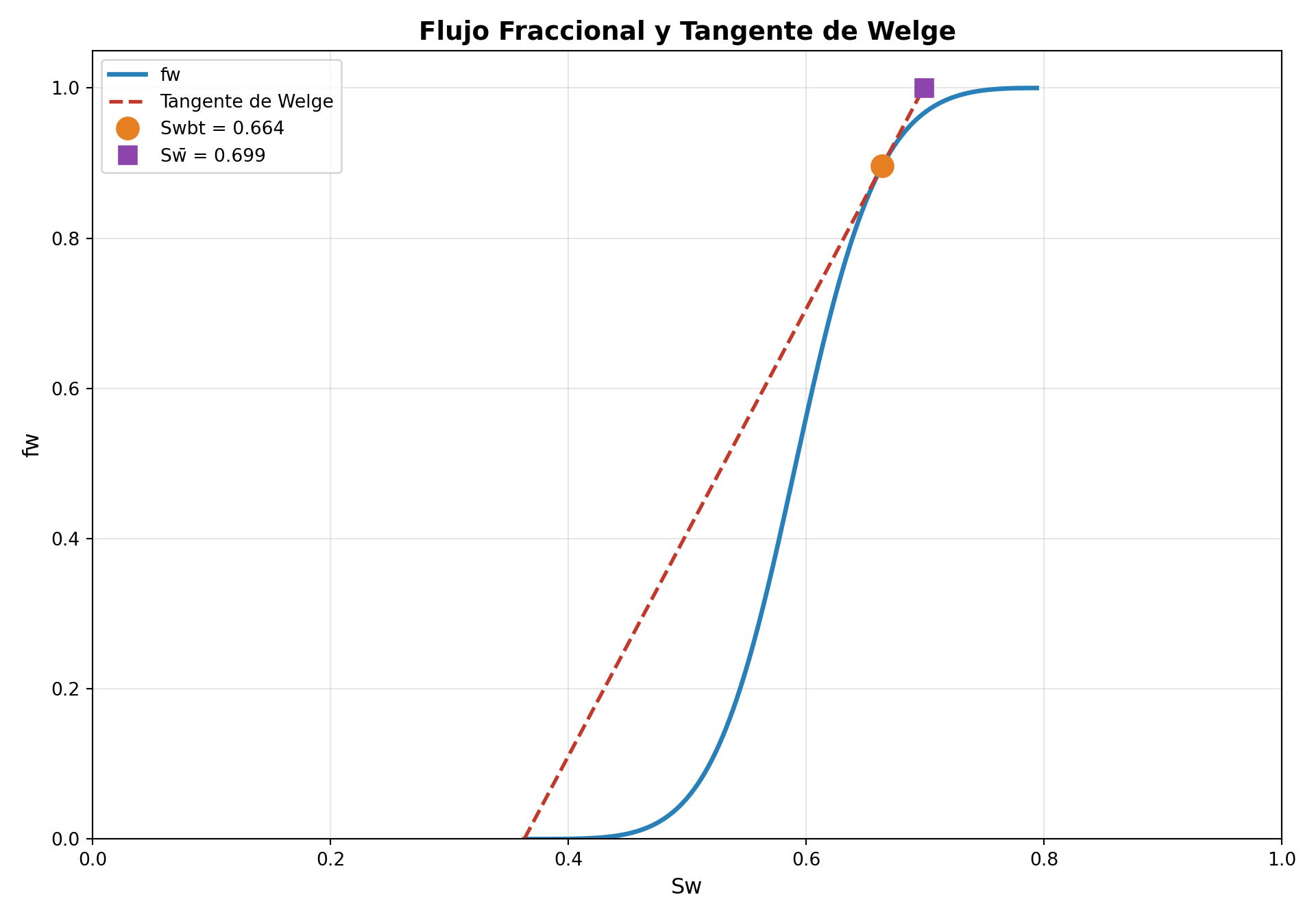
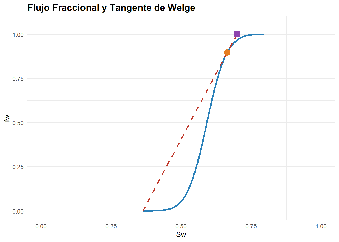
El método de Welge permite encontrar gráficamente la saturación del frente de choque (\(S_{wbt}\)): se traza una línea desde el punto \((S_{wi}, f_{wi})\) tangente a la curva de \(f_w\). El punto de tangencia define la saturación de breakthrough, y la extensión a \(f_w = 1\) da la saturación media (\(\bar{S}_w\)).

Ver código
# === FLUJO FRACCIONAL ===
A = (kromax * VisW) / (krwmax * VisO)
B_coef = 1 / (1 - Sor - Swc)

fw = SwD**nw / (SwD**nw + A * (1 - SwD)**no)
<string>:2: RuntimeWarning: invalid value encountered in power
Ver código
# Flujo fraccional en Swi
SwDi = (Swi - Swc) / (1 - Sor - Swc)
fwi = SwDi**nw / (SwDi**nw + A * (1 - SwDi)**no)

# Pendiente desde (Swi, fwi) a cada punto de la curva
slope = np.where(fw > fwi, (fw - fwi) / (Sw - Swi), 0)
<string>:3: RuntimeWarning: invalid value encountered in divide
Ver código
# Punto de breakthrough = máxima pendiente
idx_bt = np.argmax(slope)
Swbt = Sw[idx_bt]
fwbt = fw[idx_bt]
slope_max = slope[idx_bt]

# Saturación media (extensión de tangente a fw=1)
Swbt_mean = Swbt + (1/slope_max) * (1 - fwbt)

print(f"Saturación de breakthrough (Swbt): {Swbt:.4f}")
Saturación de breakthrough (Swbt): 0.6640
Ver código
print(f"fw en breakthrough:                {fwbt:.4f}")
fw en breakthrough:                0.8962
Ver código
print(f"Saturación media (Sw_mean):        {Swbt_mean:.4f}")
Saturación media (Sw_mean):        0.6989
Ver código
print(f"Pendiente máxima:                  {slope_max:.4f}")
Pendiente máxima:                  2.9773
Ver código
# === GRÁFICO ===
fig, ax = plt.subplots(figsize=(10, 7))
ax.plot(Sw, fw, '-', lw=2.5, color='#2980b9', label='fw')
ax.plot([Swi, Swbt_mean], [fwi, 1], '--', lw=2, color='#c0392b', label='Tangente de Welge')
ax.plot(Swbt, fwbt, 'o', ms=12, color='#e67e22', zorder=5, label=f'Swbt = {Swbt:.3f}')
ax.plot(Swbt_mean, 1, 's', ms=10, color='#8e44ad', zorder=5, label=f'Sw̄ = {Swbt_mean:.3f}')

ax.set_xlabel('Sw', fontsize=12); ax.set_ylabel('fw', fontsize=12)
ax.set_title('Flujo Fraccional y Tangente de Welge', fontsize=14, fontweight='bold')
ax.legend(fontsize=10); ax.grid(True, alpha=0.3)
ax.set_xlim(0, 1); ax.set_ylim(0, 1.05)
(0.0, 1.0)
(0.0, 1.05)
Ver código
plt.tight_layout(); plt.show()
Figure 3: Curva de flujo fraccional con la tangente de Welge. El punto de tangencia (●) define la saturación de breakthrough.
Ver código
A <- (kromax * VisW) / (krwmax * VisO)
B_coef <- 1/(1 - Sor - Swc)

fw <- SwD^nw / (SwD^nw + A * (1-SwD)^no)

SwDi <- (Swi - Swc) / (1 - Sor - Swc)
fwi <- SwDi^nw / (SwDi^nw + A * (1-SwDi)^no)

SLO <- ifelse(fw > fwi, (fw - fwi) / (Sw - Swi), 0)

Swbt <- Sw[which.max(SLO)]
fwbt <- fw[which.max(SLO)]
Swbt_mean <- Swbt + (1/SLO[which.max(SLO)]) * (1 - fwbt)

cat(sprintf("Swbt = %.4f, fwbt = %.4f, Sw_mean = %.4f\n", Swbt, fwbt, Swbt_mean))
Swbt = 0.6640, fwbt = 0.8962, Sw_mean = 0.6989
Ver código
ggplot() +
  geom_line(aes(x=Sw, y=fw), color="#2980b9", linewidth=1.2) +
  geom_line(aes(x=c(Swi, Swbt_mean), y=c(fwi, 1)), color="#c0392b",
            linewidth=1, linetype="dashed") +
  geom_point(aes(x=Swbt, y=fwbt), color="#e67e22", size=4) +
  geom_point(aes(x=Swbt_mean, y=1), color="#8e44ad", size=4, shape=15) +
  labs(x="Sw", y="fw", title="Flujo Fraccional y Tangente de Welge") +
  xlim(0, 1) + ylim(0, 1.05) + theme_minimal() +
  theme(plot.title=element_text(face="bold", size=14))
Figure 4: Curva de flujo fraccional con tangente de Welge.

Paso 3 — Pronóstico de Producción Post-Breakthrough

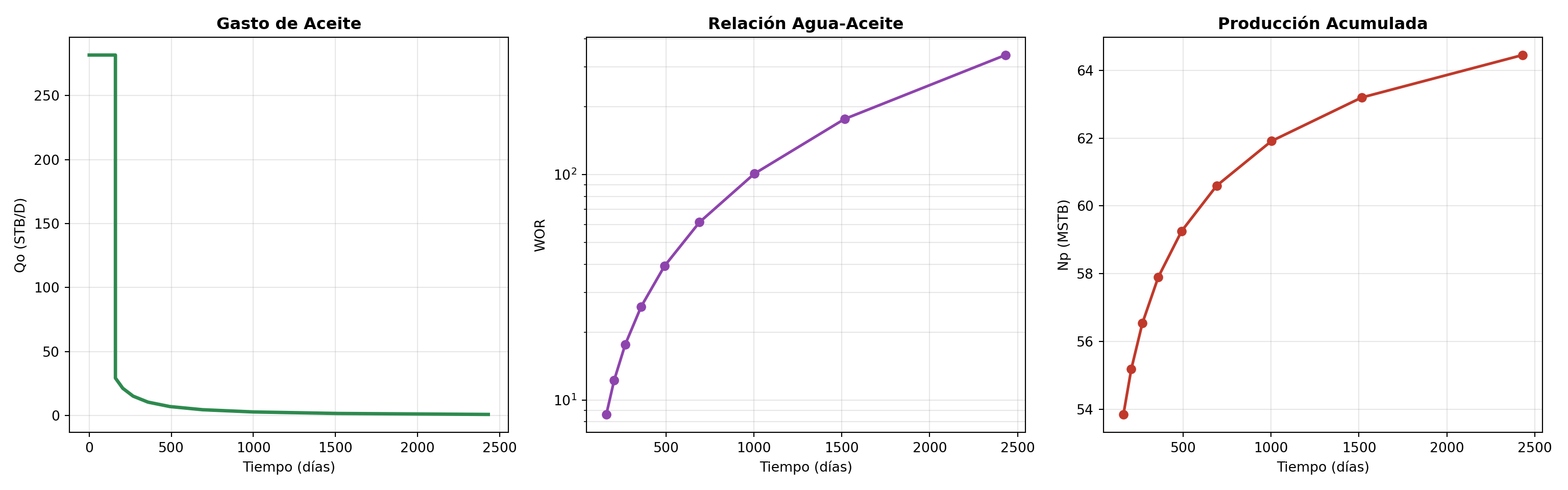
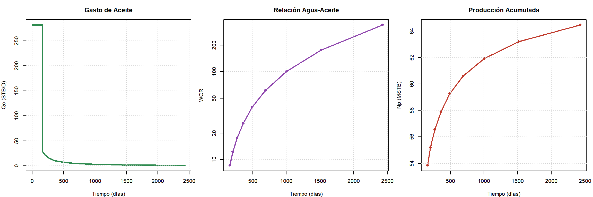
Después del breakthrough, la producción de aceite cae progresivamente y el WOR aumenta. Para cada saturación \(S_w > S_{wbt}\):

\[q_o = \frac{(1 - f_w) \cdot q_{inj}}{B_o}\]

\[WOR = \frac{f_w}{1 - f_w}\]

\[N_p = V_p \cdot (\bar{S}_w - S_{wi})\]

Ver código
# Vector de Sw después del breakthrough
SwP = np.linspace(Swbt, 0.75, 9)
SwDP = (SwP - Swc) / (1 - Sor - Swc)
krwP = krwmax * SwDP**nw
kroP = kromax * (1 - SwDP)**no

fwP = SwDP**nw / (SwDP**nw + A * (1 - SwDP)**no)

# Derivada de fw
B1 = nw * SwDP**(nw-1) * (1-SwDP)**no
B2 = no * SwDP**nw * (1-SwDP)**(no-1)
B3 = SwDP**nw + A * (1-SwDP)**no
dfw = (A * B_coef * (B1 + B2)) / B3**2

td = 1 / dfw  # Tiempo adimensional

# Saturación media
SwM = SwP + td * (1 - fwP)

# Volumen poroso
Vp = L * Ar * Poro / 5.615

# Producción
qo = ((1 - fwP) * Winj) / Bo
qw = (fwP * Winj) / Bw
WOR = fwP / (1 - fwP)
Np_cum = Vp * (SwM - Swi)
t_days = (td * Vp) / Winj

# Tabla
print(f"{'Tiempo':>8} {'Sw':>6} {'fw':>6} {'Sw_m':>6} {'Qo':>8} {'WOR':>8} {'Np':>12}")
  Tiempo     Sw     fw   Sw_m       Qo      WOR           Np
Ver código
print("-" * 60)
------------------------------------------------------------
Ver código
for i in range(len(SwP)):
    print(f"{t_days[i]:8.0f} {SwP[i]:6.3f} {fwP[i]:6.3f} {SwM[i]:6.3f} {qo[i]:8.1f} {WOR[i]:8.2f} {Np_cum[i]:12.0f}")
     160  0.664  0.896  0.699     29.2     8.63        53852
     204  0.675  0.924  0.707     21.3    12.24        55188
     268  0.686  0.946  0.716     15.1    17.65        56543
     358  0.696  0.963  0.724     10.4    25.98        57903
     491  0.707  0.975  0.733      7.0    39.27        59257
     690  0.718  0.984  0.741      4.5    61.47        60595
    1002  0.729  0.990  0.749      2.8   100.80        61910
    1515  0.739  0.994  0.757      1.6   176.34        63196
    2431  0.750  0.997  0.765      0.8   338.86        64448
Ver código
# === GRÁFICOS ===
fig, axes = plt.subplots(1, 3, figsize=(16, 5))

# Pre-BT: producción constante = Winj/Bo
t_pre = [0, t_days[0]]
qo_pre = [Winj/Bo, Winj/Bo]

axes[0].plot(t_pre + list(t_days), qo_pre + list(qo), '-', lw=2.5, color='#2d8a4e')
axes[0].set_xlabel('Tiempo (días)'); axes[0].set_ylabel('Qo (STB/D)')
axes[0].set_title('Gasto de Aceite', fontweight='bold'); axes[0].grid(True, alpha=0.3)

axes[1].semilogy(t_days, WOR, 'o-', lw=2, ms=6, color='#8e44ad')
axes[1].set_xlabel('Tiempo (días)'); axes[1].set_ylabel('WOR')
axes[1].set_title('Relación Agua-Aceite', fontweight='bold'); axes[1].grid(True, which='both', alpha=0.3)

axes[2].plot(t_days, Np_cum/1000, 'o-', lw=2, ms=6, color='#c0392b')
axes[2].set_xlabel('Tiempo (días)'); axes[2].set_ylabel('Np (MSTB)')
axes[2].set_title('Producción Acumulada', fontweight='bold'); axes[2].grid(True, alpha=0.3)

plt.tight_layout(); plt.show()
Figure 5: Pronóstico de producción: gasto de aceite y WOR después del breakthrough.
Ver código
SwP <- seq(Swbt, 0.75, length.out = 9)
SwDP <- (SwP - Swc) / (1 - Sor - Swc)

fwP <- SwDP^nw / (SwDP^nw + A * (1 - SwDP)^no)

B1 <- nw * SwDP^(nw - 1) * (1 - SwDP)^no
B2 <- no * SwDP^nw * (1 - SwDP)^(no - 1)
B3 <- SwDP^nw + A * (1 - SwDP)^no
dfw <- (A * B_coef * (B1 + B2)) / B3^2

td <- 1 / dfw
SwM <- SwP + td * (1 - fwP)
Vp <- L * Ar * Poro / 5.615

qo <- ((1 - fwP) * Winj) / Bo
qw <- (fwP * Winj) / Bw
WOR <- fwP / (1 - fwP)
Np_cum <- Vp * (SwM - Swi)
t_days <- (td * Vp) / Winj

forecast <- data.frame(
  Tiempo = round(t_days),
  Sw = round(SwP, 3),
  fw = round(fwP, 3),
  Sw_m = round(SwM, 3),
  Qo = round(qo, 1),
  WOR = round(WOR, 2),
  Np = round(Np_cum)
)

knitr::kable(forecast, caption = "Pronóstico post-breakthrough")
Table 1: Pronóstico post-breakthrough.
Pronóstico post-breakthrough
Tiempo Sw fw Sw_m Qo WOR Np
160 0.664 0.896 0.699 29.2 8.63 53852
204 0.675 0.924 0.707 21.3 12.24 55188
268 0.685 0.946 0.716 15.1 17.65 56543
358 0.696 0.963 0.724 10.4 25.98 57903
491 0.707 0.975 0.733 7.0 39.27 59257
690 0.718 0.984 0.741 4.5 61.47 60595
1002 0.728 0.990 0.749 2.8 100.80 61910
1515 0.739 0.994 0.757 1.6 176.34 63196
2431 0.750 0.997 0.765 0.8 338.86 64448
Ver código
op <- par(mfrow = c(1, 3), mar = c(4, 4, 3, 1))

# Pre-breakthrough: producción constante = Winj / Bo
t_pre <- c(0, t_days[1])
qo_pre <- c(Winj / Bo, Winj / Bo)

# 1) Gasto de aceite
plot(c(t_pre, t_days), c(qo_pre, qo),
     type = "l", lwd = 2.5, col = "#2d8a4e",
     xlab = "Tiempo (días)", ylab = "Qo (STB/D)",
     main = "Gasto de Aceite")
grid()

# 2) Relación agua-aceite
plot(t_days, WOR,
     type = "o", pch = 16, lwd = 2, col = "#8e44ad",
     log = "y",
     xlab = "Tiempo (días)", ylab = "WOR",
     main = "Relación Agua-Aceite")
grid()

# 3) Producción acumulada
plot(t_days, Np_cum / 1000,
     type = "o", pch = 16, lwd = 2, col = "#c0392b",
     xlab = "Tiempo (días)", ylab = "Np (MSTB)",
     main = "Producción Acumulada")
grid()

par(op)
Figure 6: Pronóstico post-breakthrough: gasto de aceite, relación agua-aceite y producción acumulada.

Paso 4 — Perfil de Saturación

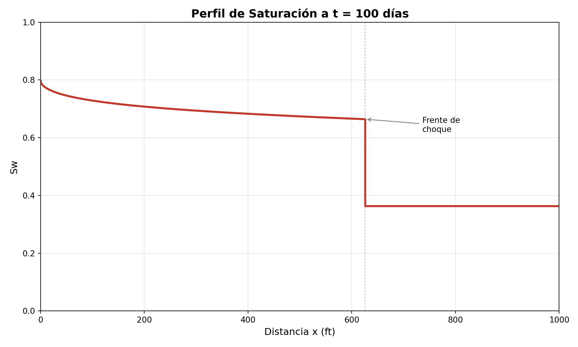
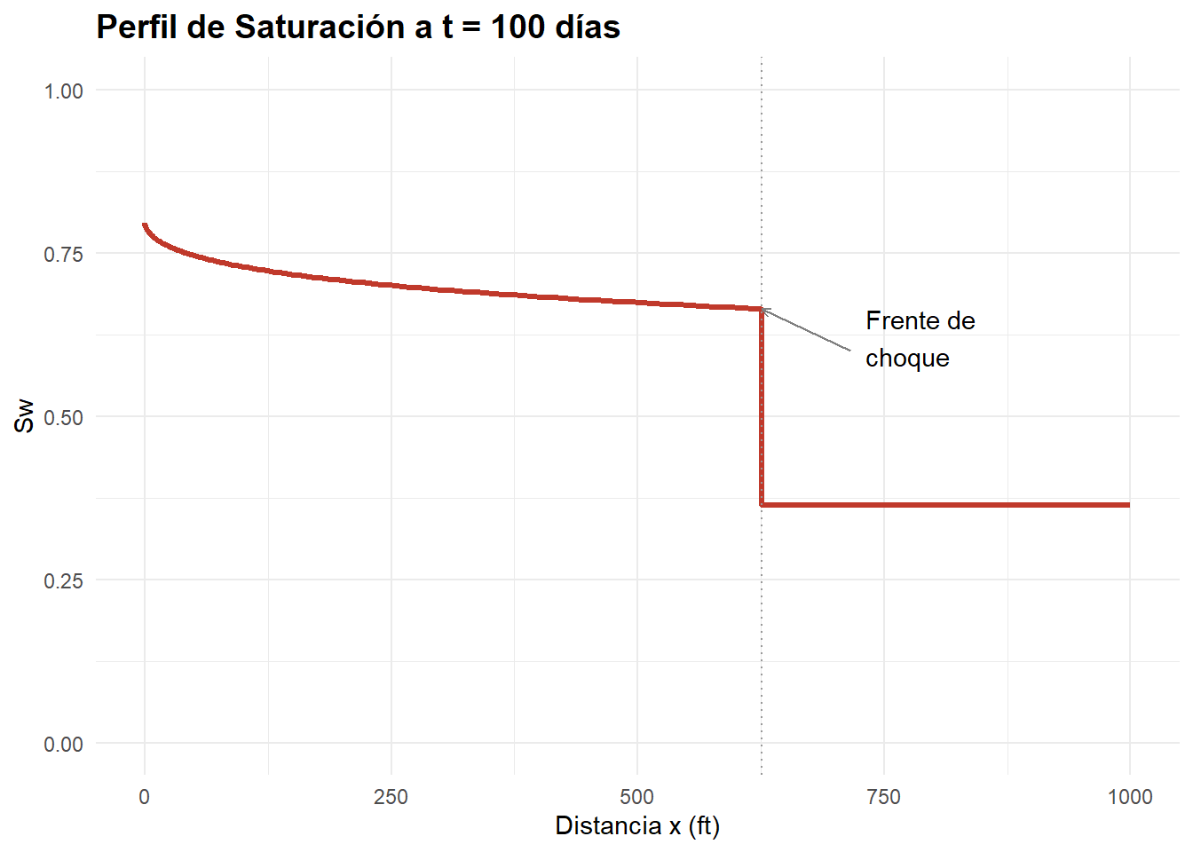
La posición de cada saturación en el yacimiento se calcula como:

\[x_{Sw} = \frac{q_t \cdot t}{A \cdot \phi} \cdot \left(\frac{\partial f_w}{\partial S_w}\right)_{Sw}\]

Ver código
days = 100

# Derivada de fw para todo el rango de Sw
SwD_all = (Sw - Swc) / (1 - Sor - Swc)
B1_all = nw * SwD_all**(nw - 1) * (1 - SwD_all)**no
B2_all = no * SwD_all**nw * (1 - SwD_all)**(no - 1)
B3_all = SwD_all**nw + A * (1 - SwD_all)**no
dfw_all = np.where(
    B3_all > 0,
    (A * B_coef * (B1_all + B2_all)) / B3_all**2,
    0
)

# Posición x(Sw)
X = dfw_all * Winj * days * 5.6146 / (Ar * Poro)

# Rama situada detrás del frente de choque
mask_front = Sw >= Swbt
x_front_branch = X[mask_front]
sw_front_branch = Sw[mask_front]

# Ordenar desde el inyector (x = 0) hasta el frente (x = xf)
order = np.argsort(x_front_branch)
x_front_branch = x_front_branch[order]
sw_front_branch = sw_front_branch[order]

# Posición del frente
xf = np.max(x_front_branch)

# Construir explícitamente el salto vertical y el tramo a Swi
x_profile = np.concatenate([x_front_branch, [xf, xf, L]])
sw_profile = np.concatenate([sw_front_branch, [Swbt, Swi, Swi]])

fig, ax = plt.subplots(figsize=(10, 6))
ax.plot(x_profile, sw_profile, '-', lw=2.5, color='#c0392b')
ax.axvline(x=xf, color='gray', ls=':', alpha=0.5)

ax.set_xlabel('Distancia x (ft)', fontsize=12)
ax.set_ylabel('Sw', fontsize=12)
ax.set_title(f'Perfil de Saturación a t = {days} días',
             fontsize=14, fontweight='bold')
ax.grid(True, alpha=0.3)
ax.set_xlim(0, L)
(0.0, 1000.0)
Ver código
ax.set_ylim(0, 1)
(0.0, 1.0)
Ver código
ax.annotate(
    'Frente de\nchoque',
    xy=(xf, Swbt),
    xytext=(xf + 110, 0.62),
    fontsize=10,
    arrowprops=dict(arrowstyle='->', color='gray')
)

plt.tight_layout()
plt.show()
Figure 7: Perfil de saturación de agua a 100 días. Se observa el frente de choque (salto discontinuo) característico de Buckley-Leverett.
Ver código
days <- 100

SwD_all <- (Sw - Swc) / (1 - Sor - Swc)
B1_all <- nw * SwD_all^(nw - 1) * (1 - SwD_all)^no
B2_all <- no * SwD_all^nw * (1 - SwD_all)^(no - 1)
B3_all <- SwD_all^nw + A * (1 - SwD_all)^no
dfw_all <- ifelse(
  B3_all > 0,
  (A * B_coef * (B1_all + B2_all)) / B3_all^2,
  0
)

X <- dfw_all * Winj * days * 5.6146 / (Ar * Poro)

mask_front <- Sw >= Swbt
x_front_branch <- X[mask_front]
sw_front_branch <- Sw[mask_front]

# Ordenar desde el inyector hasta el frente
ord <- order(x_front_branch)
x_front_branch <- x_front_branch[ord]
sw_front_branch <- sw_front_branch[ord]

xf <- max(x_front_branch)

# Incluir explícitamente el salto vertical y el tramo a Swi
perfil_df <- data.frame(
  x = c(x_front_branch, xf, xf, L),
  Sw = c(sw_front_branch, Swbt, Swi, Swi)
)

ggplot(perfil_df, aes(x = x, y = Sw)) +
  geom_line(color = "#c0392b", linewidth = 1.2) +
  geom_vline(xintercept = xf, linetype = "dotted", color = "gray60") +
  annotate(
    "segment",
    x = xf + 90, xend = xf,
    y = 0.60, yend = Swbt,
    arrow = arrow(length = grid::unit(0.15, "cm")),
    color = "gray50"
  ) +
  annotate(
    "text",
    x = xf + 105, y = 0.62,
    label = "Frente de\nchoque",
    hjust = 0
  ) +
  labs(
    x = "Distancia x (ft)",
    y = "Sw",
    title = sprintf("Perfil de Saturación a t = %d días", days)
  ) +
  xlim(0, L) +
  ylim(0, 1) +
  theme_minimal() +
  theme(plot.title = element_text(face = "bold", size = 14))
Figure 8: Perfil de saturación de agua a 100 días. Se observa el frente de choque característico de Buckley-Leverett.

Resumen de Resultados

Parámetro Valor
Saturación de breakthrough (\(S_{wbt}\)) El valor calculado
fw en breakthrough El valor calculado
Saturación media (\(\bar{S}_w\)) El valor calculado
Eficiencia de desplazamiento \(E_D = (\bar{S}_w - S_{wi}) / (1 - S_{or} - S_{wi})\)

Referencias

  • Buckley, S.E. & Leverett, M.C. (1942). Mechanism of Fluid Displacement in Sands. Trans. AIME, 146.
  • Welge, H.J. (1952). A Simplified Method for Computing Oil Recovery by Gas or Water Drive. Trans. AIME, 195.
  • Ahmed, T. (2019). Reservoir Engineering Handbook, 5th ed. Gulf Professional Publishing. Cap. 14.
  • Wu, Y-S. (2016). Multiphase Fluid Flow in Porous and Fractured Reservoirs. Elsevier.

🛒
Propiedades De Los Fluidos Del Yacimiento

Disponible en Mercado Libre

Ver oferta →