Curvas IPR Compuestas: Pozos con Producción de Agua
Método Composite IPR de Brown (1984) en R, Python y Excel
Yacimientos
Producción
R
Python
Excel
Cuando un pozo produce aceite y agua simultáneamente, la curva IPR clásica de Vogel no es suficiente. Aprende a construir la curva IPR compuesta (Composite IPR) que combina Vogel para aceite y PI constante para agua.
¿Por qué una IPR Compuesta?
La curva IPR de Vogel funciona muy bien para pozos que producen solo aceite en yacimientos por debajo de la presión de burbuja. Pero en la realidad, muchos pozos producen aceite y agua simultáneamente, y el comportamiento de cada fluido es diferente:
- Aceite: En yacimientos subsaturados (\(P_{wf} < P_b\)), la relación presión-gasto es no lineal (Vogel)
- Agua: Sigue una relación lineal con índice de productividad constante (\(J\))
El método de IPR Compuesta (Composite IPR), propuesto por Brown (1984), combina ambos comportamientos en una sola curva usando la fracción de agua (\(F_w\)) como ponderador.
¿Cuándo usar este método?
Úsalo cuando tu pozo produce agua con un corte de agua significativo (\(F_w > 0\)) y necesitas generar la curva IPR para diseño de levantamiento artificial o análisis nodal.
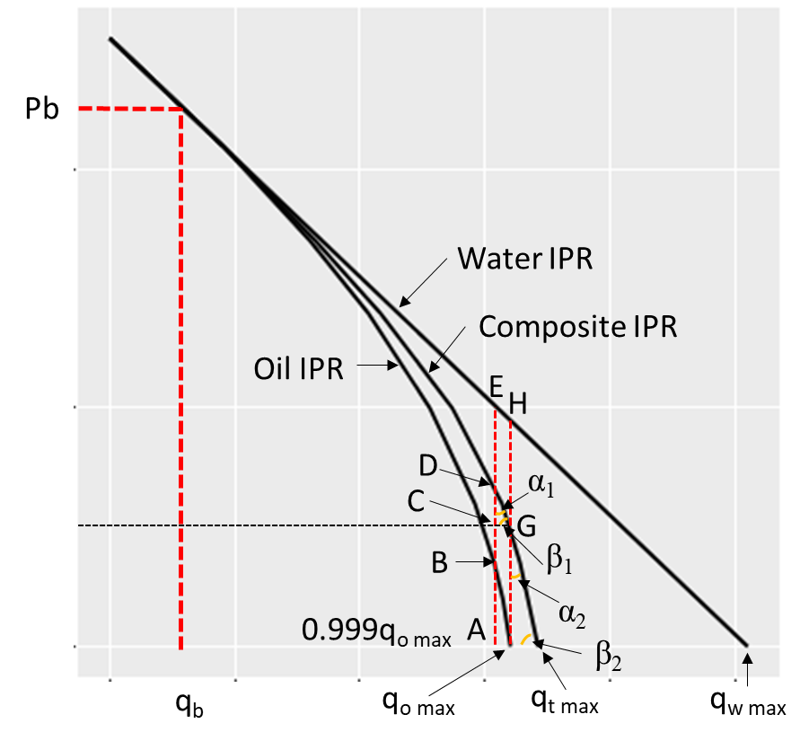
Las Tres Regiones de la Curva
La curva IPR compuesta se divide en 3 regiones, cada una con su ecuación:
Región 1: \(P_b < P_{wf} < P_r\) (Monofásica)
Por encima de la presión de burbuja, solo hay flujo monofásico. La relación es lineal:
\[q_t = J(P_r - P_{wf})\]
Región 2: \(P_{wfG} < P_{wf} < P_b\) (Bifásica)
Entre la presión de burbuja y la presión donde el aceite alcanza su gasto máximo. Aquí se combinan Vogel (aceite) y PI lineal (agua):
Para \(B \neq 0\):
\[q_t = \frac{-C + \sqrt{C^2 - 4B^2D}}{2B^2}\]
Donde:
\[A = \frac{P_{wf} + 0.125 \cdot F_o \cdot P_b - F_w \cdot P_r}{0.125 \cdot F_o \cdot P_b}\]
\[B = \frac{F_w}{0.125 \cdot F_o \cdot P_b \cdot J}\]
\[C = 2AB + \frac{80}{q_{omax} - q_b}\]
\[D = A^2 - 80 \cdot \frac{q_b}{q_{omax} - q_b} - 81\]
Con \(F_o = 1 - F_w\).
Región 3: \(0 < P_{wf} < P_{wfG}\) (Extensión lineal)
Debajo de la presión donde el aceite llega a su máximo, la curva se extiende linealmente usando \(\tan\beta\):
\[q_t = \frac{P_{wfG} + q_{omax} \cdot \tan\beta - P_{wf}}{\tan\beta}\]
Datos del Ejemplo
| Parámetro | Valor | Unidades |
|---|---|---|
| Presión de yacimiento (\(P_r\)) | 2,550 | psi |
| Presión de burbuja (\(P_b\)) | 2,100 | psi |
| Presión de fondo fluyente (prueba) | 2,300 | psi |
| Gasto total (prueba) | 500 | b/d |
| Fracción de agua (\(F_w\)) | 0.50 | — |
Parámetros Calculados
A partir de los datos de la prueba se calculan los parámetros base:
| Parámetro | Fórmula | Valor |
|---|---|---|
| Índice de productividad (\(J\)) | \(q_{test} / (P_r - P_{wf,test})\) | 2.0 b/d/psi |
| Gasto al punto de burbuja (\(q_b\)) | \(J \cdot (P_r - P_b)\) | 900 b/d |
| Gasto máximo de aceite (\(q_{omax}\)) | \(q_b + J \cdot P_b / 1.8\) | 3,233.33 b/d |
| Presión en \(q_{omax}\) (\(P_{wfG}\)) | \(F_w(P_r - q_{omax}/J)\) | 466.67 psi |
| Gasto máximo total (\(q_{tmax}\)) | \(q_{omax} + F_w(P_r - q_{omax}/J) \cdot \tan\alpha\) | Calculado |
Código: R y Python
Ver código
import numpy as np
import matplotlib.pyplot as plt

# === DATOS DE ENTRADA ===
Pr = 2550       # Presión de yacimiento (psi)
Pb = 2100       # Presión de burbuja (psi)
Pwf_test = 2300 # Pwf de la prueba (psi)
Qt_test = 500   # Gasto total de la prueba (b/d)
Fw = 0.5        # Fracción de agua
Fo = 1 - Fw     # Fracción de aceite

# === PARÁMETROS CALCULADOS ===
J = Qt_test / (Pr - Pwf_test)               # Índice de productividad
qb = J * (Pr - Pb)                           # Gasto al punto de burbuja
qomax = qb + J * Pb / 1.8                    # Gasto máximo de aceite

# Cálculo de tan(alpha) y tan(beta)
CD = (Fo * 0.125 * Pb * (np.sqrt(81 - 80 * (0.999 * qomax - qb) / (qomax - qb)) - 1)
      + Fw * (Pr - (0.999 * qomax) / J) - Fw * (Pr - qomax / J))
CG = 0.001 * qomax
tan_a = CG / CD
tan_b = 1 / tan_a

# Presión y gasto máximo total
PwfG = Fw * (Pr - qomax / J)
qtmax = qomax + Fw * (Pr - qomax / J) * tan_a

print(f"J       = {J:.2f} b/d/psi")
J = 2.00 b/d/psiVer código
print(f"qb = {qb:.2f} b/d")qb = 900.00 b/dVer código
print(f"qomax = {qomax:.2f} b/d")qomax = 3233.33 b/dVer código
print(f"PwfG = {PwfG:.2f} psi")PwfG = 466.67 psiVer código
print(f"tan(α) = {tan_a:.4f}")tan(α) = 0.4097Ver código
print(f"tan(β) = {tan_b:.4f}")tan(β) = 2.4409Ver código
print(f"qtmax = {qtmax:.2f} b/d")qtmax = 3424.52 b/dVer código
# === FUNCIONES AUXILIARES ===
def calc_A(Pwf, Fo, Pb, Pr, Fw):
    return (Pwf + 0.125 * Fo * Pb - Fw * Pr) / (0.125 * Fo * Pb)

def calc_B(Fw, Fo, Pb, J):
    return Fw / (0.125 * Fo * Pb * J)

def calc_C(A, B, qomax, qb):
    return 2 * A * B + 80 / (qomax - qb)

def calc_D(A, qb, qomax):
    return A**2 - 80 * (qb / (qomax - qb)) - 81

# === CALCULAR IPR COMPUESTA ===
pwf_vec = np.array([0, 200, 350, 600, 1000, 1400, 1500, 1700, 2100, 2300, 2400, 2550])

qt_vec = np.zeros_like(pwf_vec, dtype=float)

for i, pwf in enumerate(pwf_vec):
    if pwf >= Pb:
        # Región 1: Lineal (monofásica)
        qt_vec[i] = J * (Pr - pwf)
    elif pwf >= PwfG:
        # Región 2: Bifásica (Vogel + PI)
        A = calc_A(pwf, Fo, Pb, Pr, Fw)
        B = calc_B(Fw, Fo, Pb, J)
        C = calc_C(A, B, qomax, qb)
        D = calc_D(A, qb, qomax)
        if B != 0:
            qt_vec[i] = (-C + np.sqrt(C**2 - 4 * B**2 * D)) / (2 * B**2)
        else:
            qt_vec[i] = -D / C
    else:
        # Región 3: Extensión lineal
        qt_vec[i] = (PwfG + qomax * tan_b - pwf) / tan_b

# === TABLA DE RESULTADOS ===
print(f"{'Pwf (psi)':>10} {'qt (b/d)':>12}")
Pwf (psi) qt (b/d)Ver código
print("-" * 24)------------------------Ver código
for p, q in zip(pwf_vec, qt_vec):
    print(f"{p:10.0f} {q:12.2f}")
0 3424.52
200 3342.58
350 3281.13
600 3159.86
1000 2758.15
1400 2177.33
1500 2012.26
1700 1662.93
2100 900.00
2300 500.00
2400 300.00
2550 0.00Ver código
# === GRÁFICO ===
# Para evitar quiebres numéricos en los cambios de región,
# se construye la curva por segmentos e incluyendo exactamente Pb y PwfG.

def qt_composite_single(pwf):
    if pwf >= Pb:
        return J * (Pr - pwf)
    elif pwf >= PwfG:
        A = calc_A(pwf, Fo, Pb, Pr, Fw)
        B = calc_B(Fw, Fo, Pb, J)
        C = calc_C(A, B, qomax, qb)
        D = calc_D(A, qb, qomax)
        discriminant = max(C**2 - 4 * B**2 * D, 0)
        if B != 0:
            return (-C + np.sqrt(discriminant)) / (2 * B**2)
        return -D / C
    else:
        return (PwfG + qomax * tan_b - pwf) / tan_b

pwf_reg3 = np.linspace(0, PwfG, 80)
pwf_reg2 = np.linspace(PwfG, Pb, 120)
pwf_reg1 = np.linspace(Pb, Pr, 80)
pwf_smooth = np.unique(np.concatenate([pwf_reg3, pwf_reg2, pwf_reg1]))
qt_smooth = np.array([qt_composite_single(p) for p in pwf_smooth])

fig, ax = plt.subplots(figsize=(10, 7))
ax.plot(qt_smooth, pwf_smooth, '-', lw=2.5, color='#2d8a4e', label=f'Composite IPR (Fw={Fw})')
ax.plot(qt_vec, pwf_vec, 'o', ms=6, color='#c0392b', label='Puntos calculados', zorder=5)

# Líneas de referencia
ax.axhline(y=Pb, color='gray', ls='--', alpha=0.5, lw=0.8)
ax.text(100, Pb + 30, f'Pb = {Pb} psi', fontsize=9, color='gray')
ax.axhline(y=PwfG, color='gray', ls='--', alpha=0.5, lw=0.8)
ax.text(100, PwfG + 30, f'PwfG = {PwfG:.0f} psi', fontsize=9, color='gray')

# Puntos especiales
ax.plot(qb, Pb, 's', ms=10, color='#e67e22', zorder=6)
ax.annotate(f'qb = {qb:.0f}', xy=(qb, Pb), xytext=(qb+200, Pb+100),
            fontsize=9, arrowprops=dict(arrowstyle='->', color='#e67e22'), color='#e67e22')
ax.plot(qomax, PwfG, 's', ms=10, color='#8e44ad', zorder=6)
ax.annotate(f'qomax = {qomax:.0f}', xy=(qomax, PwfG), xytext=(qomax-800, PwfG+200),
            fontsize=9, arrowprops=dict(arrowstyle='->', color='#8e44ad'), color='#8e44ad')

ax.set_xlabel('Gasto total, qt (b/d)', fontsize=12)
ax.set_ylabel('Presión de fondo fluyente, Pwf (psi)', fontsize=12)
ax.set_title('Curva IPR Compuesta — Método de Brown (1984)', fontsize=14, fontweight='bold')
ax.legend(fontsize=10)
ax.grid(True, alpha=0.3)
ax.set_xlim(left=0)
(0.0, 3595.747525657348)Ver código
ax.set_ylim(bottom=0)(0.0, 2677.5)Ver código
plt.tight_layout()
plt.show()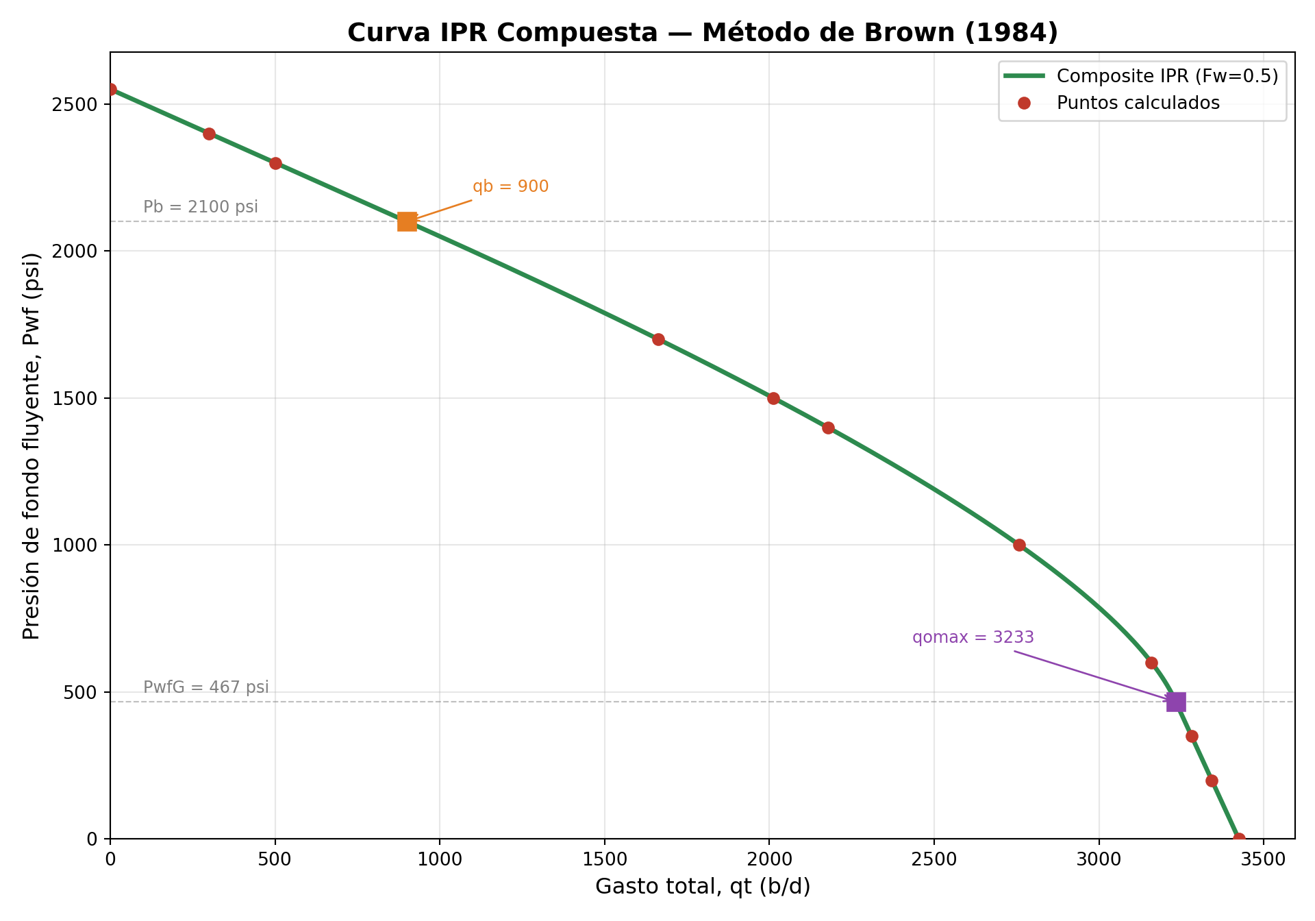
Ver código
library(ggplot2)

# === DATOS DE ENTRADA ===
Pr <- 2550       # Presión de yacimiento (psi)
Pb <- 2100       # Presión de burbuja (psi)
Pwf_test <- 2300 # Pwf de la prueba (psi)
Qt_test <- 500   # Gasto total de la prueba (b/d)
Fw <- 0.5        # Fracción de agua
Fo <- 1 - Fw     # Fracción de aceite

# === PARÁMETROS CALCULADOS ===
J <- Qt_test / (Pr - Pwf_test)
qb <- J * (Pr - Pb)
qomax <- qb + J * Pb / 1.8

CD <- Fo * 0.125 * Pb * (sqrt(81 - 80 * (0.999 * qomax - qb) / (qomax - qb)) - 1) +
      Fw * (Pr - (0.999 * qomax) / J) - Fw * (Pr - qomax / J)
CG <- 0.001 * qomax
tana <- CG / CD
tanb <- 1 / tana

PwfG <- Fw * (Pr - qomax / J)
qtmax <- qomax + Fw * (Pr - qomax / J) * tana

cat(sprintf("J       = %.2f b/d/psi\n", J))
J = 2.00 b/d/psiVer código
cat(sprintf("qb = %.2f b/d\n", qb))qb = 900.00 b/dVer código
cat(sprintf("qomax = %.2f b/d\n", qomax))qomax = 3233.33 b/dVer código
cat(sprintf("PwfG = %.2f psi\n", PwfG))PwfG = 466.67 psiVer código
cat(sprintf("tan(α) = %.4f\n", tana))tan(α) = 0.4097Ver código
cat(sprintf("tan(β) = %.4f\n", tanb))tan(β) = 2.4409Ver código
cat(sprintf("qtmax = %.2f b/d\n", qtmax))qtmax = 3424.52 b/dVer código
# === FUNCIONES AUXILIARES ===
A_IPR_c <- function(Pwf, Fw, Pb, Pr) {
  Fo <- 1 - Fw
  (Pwf + 0.125 * Fo * Pb - Fw * Pr) / (0.125 * Fo * Pb)
}

B_IPR_c <- function(Fw, Pb, J) {
  Fo <- 1 - Fw
  Fw / (0.125 * Fo * Pb * J)
}

C_IPR_c <- function(Pwf, Fw, Pb, Pr, J, qomax, qb) {
  A <- A_IPR_c(Pwf, Fw, Pb, Pr)
  B <- B_IPR_c(Fw, Pb, J)
  2 * A * B + 80 / (qomax - qb)
}

D_IPR_c <- function(Pwf, Fw, Pb, Pr, J, qomax, qb) {
  A <- A_IPR_c(Pwf, Fw, Pb, Pr)
  A^2 - 80 * (qb / (qomax - qb)) - 81
}

# === CALCULAR IPR COMPUESTA ===
pwf <- c(0, 200, 350, 600, 1000, 1400, 1500, 1700, 2100, 2300, 2400, 2550)

A <- A_IPR_c(pwf, Fw, Pb, Pr)
B <- B_IPR_c(Fw, Pb, J)
C <- C_IPR_c(pwf, Fw, Pb, Pr, J, qomax, qb)
D <- D_IPR_c(pwf, Fw, Pb, Pr, J, qomax, qb)

qt <- ifelse(pwf >= Pb, J * (Pr - pwf),
        ifelse(pwf >= PwfG & pwf < Pb,
          ifelse(rep(B, length(pwf)) != 0,
                 (-C + sqrt(C^2 - 4 * B^2 * D)) / (2 * B^2), -D / C),
          ifelse(pwf < PwfG, (PwfG + qomax * tanb - pwf) / tanb, 0)))

IPR <- data.frame(pwf = pwf, qt = qt)

# === GRÁFICO ===
ggplot(IPR, aes(x = qt, y = pwf)) +
  geom_line(color = "#2d8a4e", linewidth = 1.2) +
  geom_point(color = "#c0392b", size = 3) +
  geom_hline(yintercept = Pb, linetype = "dashed", color = "gray", alpha = 0.6) +
  geom_hline(yintercept = PwfG, linetype = "dashed", color = "gray", alpha = 0.6) +
  annotate("text", x = 100, y = Pb + 40, label = paste("Pb =", Pb, "psi"),
           color = "gray", size = 3.5) +
  annotate("text", x = 100, y = PwfG + 40, label = paste("PwfG =", round(PwfG), "psi"),
           color = "gray", size = 3.5) +
  labs(x = "Gasto total, qt (b/d)",
       y = "Presión de fondo fluyente, Pwf (psi)",
       title = "Curva IPR Compuesta — Método de Brown (1984)") +
  theme_minimal() +
  theme(plot.title = element_text(face = "bold", size = 14))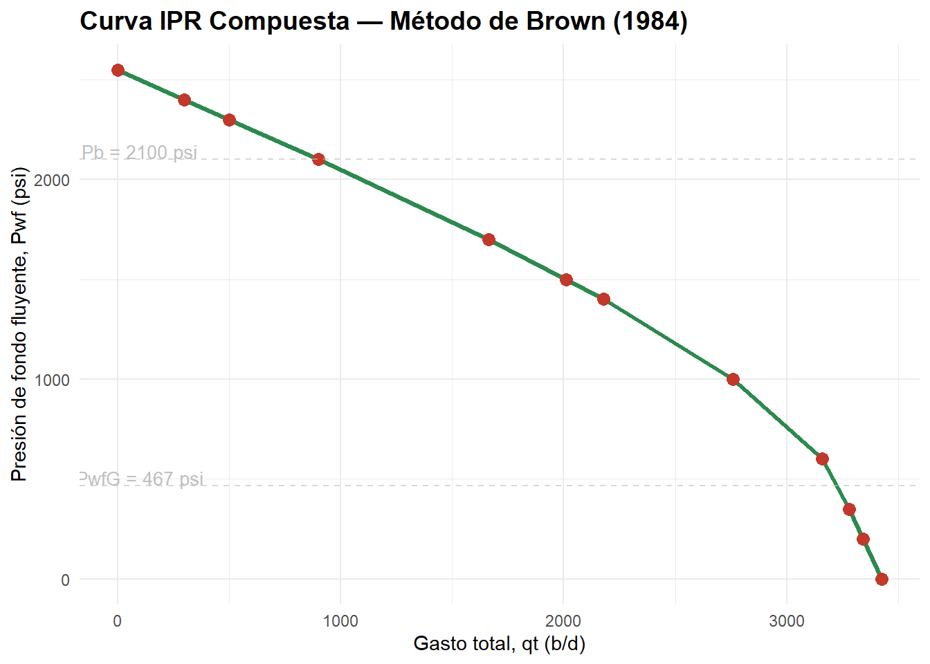
Ver código
knitr::kable(IPR, col.names = c("Pwf (psi)", "qt (b/d)"),
caption = "Composite IPR, Fw = 0.5", digits = 2)| Pwf (psi) | qt (b/d) |
|---|---|
| 0 | 3424.52 |
| 200 | 3342.58 |
| 350 | 3281.13 |
| 600 | 3159.86 |
| 1000 | 2758.15 |
| 1400 | 2177.33 |
| 1500 | 2012.26 |
| 1700 | 1662.93 |
| 2100 | 900.00 |
| 2300 | 500.00 |
| 2400 | 300.00 |
| 2550 | 0.00 |
Cómo Hacerlo en Excel
El mismo cálculo se puede replicar en Excel sin macros:
Paso 1 — Datos de entrada
Coloca los datos en celdas fijas:
| Celda | Contenido | Valor |
|---|---|---|
| B1 | \(P_r\) | 2550 |
| B2 | \(P_b\) | 2100 |
| B3 | \(P_{wf,test}\) | 2300 |
| B4 | \(q_{t,test}\) | 500 |
| B5 | \(F_w\) | 0.5 |
Paso 2 — Parámetros calculados
| Celda | Fórmula | Resultado |
|---|---|---|
| B7 (\(J\)) | =B4/(B1-B3) |
2.00 |
| B8 (\(q_b\)) | =B7*(B1-B2) |
900 |
| B9 (\(q_{omax}\)) | =B8+B7*B2/1.8 |
3,233.33 |
| B10 (\(F_o\)) | =1-B5 |
0.50 |
| B11 (\(P_{wfG}\)) | =B5*(B1-B9/B7) |
458.33 |
Paso 3 — Tabla de cálculo
Crea una columna de \(P_{wf}\) (de 0 a \(P_r\)) y usa la función SI() anidada para calcular \(q_t\) según la región:
=SI(A13>=B2, B7*(B1-A13),
  SI(A13>=B11,
    SI(D13<>0,(-C13+RAIZ(C13^2-4*D13^2*E13))/(2*D13^2),-E13/C13),
    (B11+B9*F13-A13)/F13))
Donde C13, D13, E13 y F13 son las columnas auxiliares con los valores de C, B, D y \(\tan\beta\) respectivamente.
📸 IMAGEN: Captura de la hoja de Excel mostrando: datos de entrada (B1:B5), parámetros calculados (B7:B11), tabla de Pwf vs qt con fórmulas, y el gráfico XY de la curva IPR resultante.
Paso 4 — Gráfico
- Seleccionar columnas qt (eje X) y Pwf (eje Y)
- Insertar → Gráfico de Dispersión con Líneas
- Agregar líneas horizontales punteadas en \(P_b\) y \(P_{wfG}\)
- Formato: título, etiquetas de ejes, gridlines
Análisis de Sensibilidad: Efecto de \(F_w\)
Un ejercicio muy útil es generar la curva IPR para diferentes valores de \(F_w\) y observar cómo el incremento de agua afecta la productividad del pozo.
Ver código
fig, ax = plt.subplots(figsize=(10, 7))

fw_values = [0.0, 0.25, 0.50, 0.75]
colors_fw = ['#2d8a4e', '#2980b9', '#e67e22', '#c0392b']

def composite_ipr_curve(fw, n=250):
    """Calcula qt(Pwf) para la IPR compuesta evitando discontinuidades numéricas."""
    fo = 1 - fw
    qb_s = J * (Pr - Pb)
    qomax_s = qb_s + J * Pb / 1.8
    pwf_s = np.linspace(0, Pr, n)
    qt_s = np.zeros_like(pwf_s)

    # Caso límite: solo aceite -> Vogel bajo Pb + línea sobre Pb
    if np.isclose(fw, 0):
        for i, p in enumerate(pwf_s):
            if p >= Pb:
                qt_s[i] = J * (Pr - p)
            else:
                r = p / Pb
                qt_s[i] = qb_s + (qomax_s - qb_s) * (1 - 0.2 * r - 0.8 * r**2)
        return pwf_s, qt_s

    CD_s = (fo * 0.125 * Pb * (np.sqrt(81 - 80 * (0.999 * qomax_s - qb_s) / (qomax_s - qb_s)) - 1)
            + fw * (Pr - (0.999 * qomax_s) / J) - fw * (Pr - qomax_s / J))
    tan_a_s = (0.001 * qomax_s) / CD_s
    tan_b_s = 1 / tan_a_s
    PwfG_s = fw * (Pr - qomax_s / J)

    for i, p in enumerate(pwf_s):
        if p >= Pb:
            qt_s[i] = J * (Pr - p)
        elif p >= PwfG_s:
            A = (p + 0.125 * fo * Pb - fw * Pr) / (0.125 * fo * Pb)
            B = fw / (0.125 * fo * Pb * J)
            C = 2 * A * B + 80 / (qomax_s - qb_s)
            D = A**2 - 80 * (qb_s / (qomax_s - qb_s)) - 81
            disc = max(C**2 - 4 * B**2 * D, 0)
            qt_s[i] = (-C + np.sqrt(disc)) / (2 * B**2)
        else:
            qt_s[i] = (PwfG_s + qomax_s * tan_b_s - p) / tan_b_s

    return pwf_s, qt_s

for fw, color in zip(fw_values, colors_fw):
    pwf_s, qt_s = composite_ipr_curve(fw)
    ax.plot(qt_s, pwf_s, '-', lw=2, color=color, label=f'Fw = {fw}')

ax.set_xlabel('Gasto total, qt (b/d)', fontsize=12)
ax.set_ylabel('Pwf (psi)', fontsize=12)
ax.set_title('Análisis de Sensibilidad — Efecto de Fw', fontsize=14, fontweight='bold')
ax.legend(fontsize=11)
ax.grid(True, alpha=0.3)
ax.set_xlim(left=0)
(0.0, 3894.8509102138864)Ver código
ax.set_ylim(bottom=0)(0.0, 2677.5)Ver código
plt.tight_layout()
plt.show()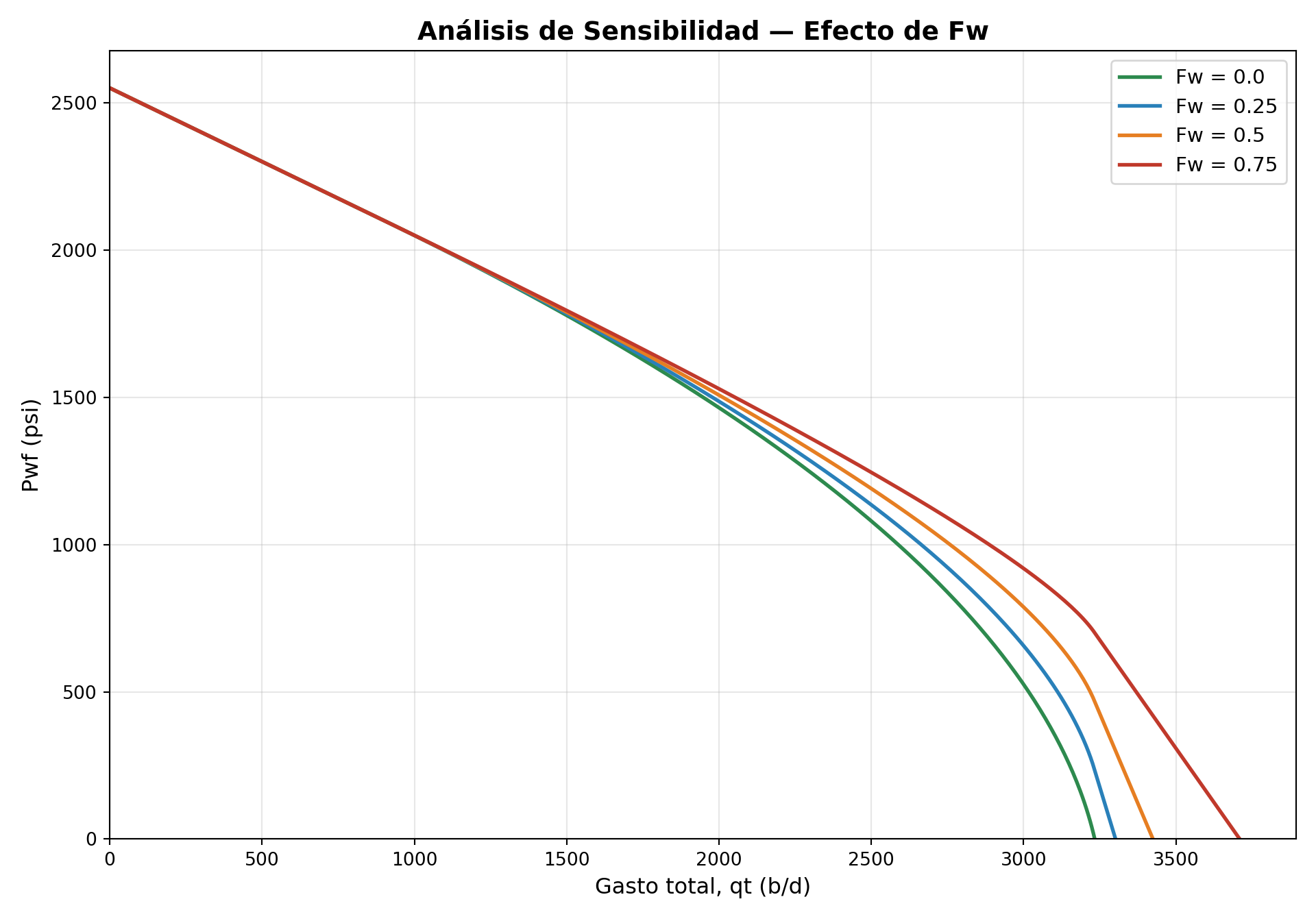
Ver código
fw_values <- c(0.0, 0.25, 0.50, 0.75)

calc_composite_ipr <- function(fw_val, n = 250) {
  fo_val <- 1 - fw_val
  qb_s <- J * (Pr - Pb)
  qomax_s <- qb_s + J * Pb / 1.8
  pwf_s <- seq(0, Pr, length.out = n)
  qt_s <- numeric(length(pwf_s))

  # Caso límite: solo aceite -> Vogel bajo Pb + línea sobre Pb
  if (isTRUE(all.equal(fw_val, 0))) {
    for (i in seq_along(pwf_s)) {
      p <- pwf_s[i]
      if (p >= Pb) {
        qt_s[i] <- J * (Pr - p)
      } else {
        r <- p / Pb
        qt_s[i] <- qb_s + (qomax_s - qb_s) * (1 - 0.2 * r - 0.8 * r^2)
      }
    }
    return(data.frame(pwf = pwf_s, qt = qt_s, Fw = factor(fw_val)))
  }

  CD_s <- fo_val * 0.125 * Pb *
    (sqrt(81 - 80 * (0.999 * qomax_s - qb_s) / (qomax_s - qb_s)) - 1) +
    fw_val * (Pr - (0.999 * qomax_s) / J) -
    fw_val * (Pr - qomax_s / J)

  tana_s <- (0.001 * qomax_s) / CD_s
  tanb_s <- 1 / tana_s
  PwfG_s <- fw_val * (Pr - qomax_s / J)

  for (i in seq_along(pwf_s)) {
    p <- pwf_s[i]

    if (p >= Pb) {
      qt_s[i] <- J * (Pr - p)
    } else if (p >= PwfG_s) {
      A_s <- (p + 0.125 * fo_val * Pb - fw_val * Pr) / (0.125 * fo_val * Pb)
      B_s <- fw_val / (0.125 * fo_val * Pb * J)
      C_s <- 2 * A_s * B_s + 80 / (qomax_s - qb_s)
      D_s <- A_s^2 - 80 * (qb_s / (qomax_s - qb_s)) - 81
      disc <- max(C_s^2 - 4 * B_s^2 * D_s, 0)
      qt_s[i] <- (-C_s + sqrt(disc)) / (2 * B_s^2)
    } else {
      qt_s[i] <- (PwfG_s + qomax_s * tanb_s - p) / tanb_s
    }
  }

  data.frame(pwf = pwf_s, qt = qt_s, Fw = factor(fw_val))
}

all_data <- do.call(rbind, lapply(fw_values, calc_composite_ipr))

ggplot(all_data, aes(x = qt, y = pwf, color = Fw, group = Fw)) +
  geom_line(linewidth = 1.2) +
  scale_color_manual(values = c("#2d8a4e", "#2980b9", "#e67e22", "#c0392b")) +
  labs(x = "Gasto total, qt (b/d)", y = "Pwf (psi)",
       title = "Análisis de Sensibilidad — Efecto de Fw",
       color = "Fw") +
  theme_minimal() +
  theme(plot.title = element_text(face = "bold", size = 14))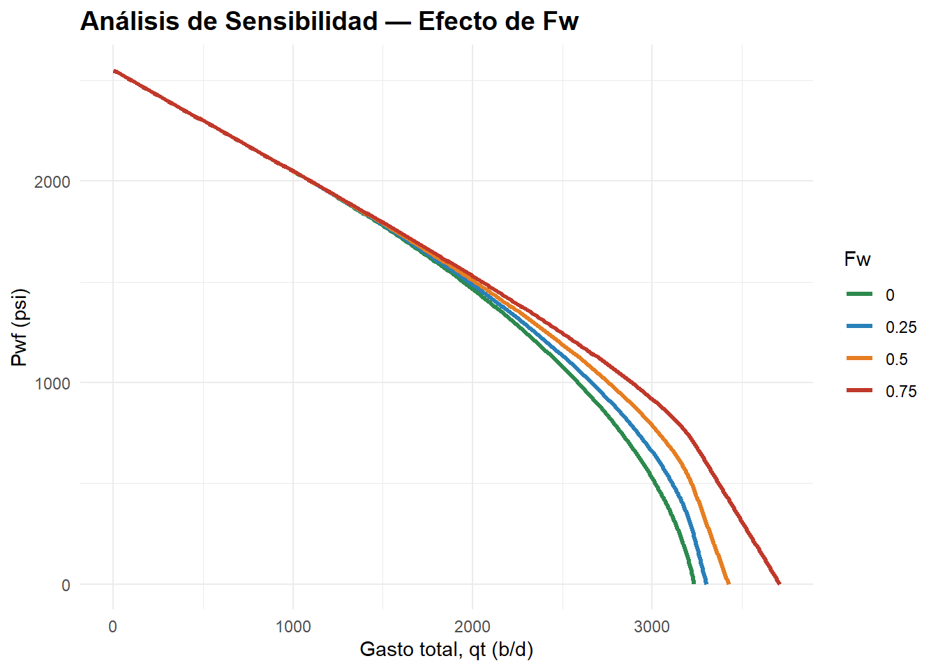
Observaciones del análisis de sensibilidad:
- Con \(F_w = 0\) (solo aceite), la curva es la IPR de Vogel clásica
- A medida que \(F_w\) aumenta, la curva se “estira” hacia la derecha: el gasto máximo total aumenta pero gran parte es agua
- La curvatura de la zona bifásica se atenúa con mayor \(F_w\) porque el componente lineal del agua domina
- En el extremo \(F_w = 1\) (solo agua), la IPR sería una línea recta con pendiente \(1/J\)
Referencias
- Brown, K.E. (1984). The Technology of Artificial Lift Methods, Vol. 4. PennWell Books.
- Vogel, J.V. (1968). Inflow Performance Relationships for Solution-Gas Drive Wells. JPT, 20(1).